What are Autoencoders?

Autoencoders are unsupervised neural networks that "learn" compressed representations of their input data. Their goal is to reduce the dimensionality of their input in such a way that it can still be accurately reconstructed. It finds useful representations of its input by taking advantage of existing patterns in the data it is trained on.

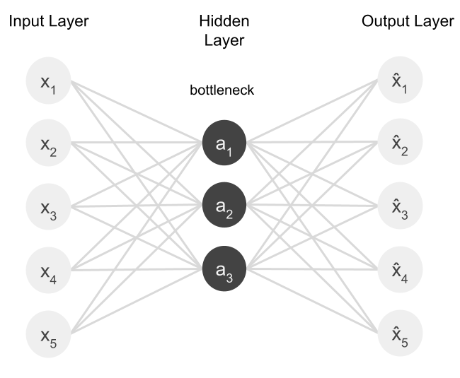
The autoencoder has three main parts:

1. An encoder, which reduces the dimensionality of the input data.
2. The bottleneck, which stores the compressed representations of the input data.
3. The decoder, which attempts to recreate the input data from its encoded, dimension-reduced form.

What are Autoencoders Used For?

In the past, autoencoders primarily had one of two purposes: feature extraction or dimension reduction. Both are performed at the same time. Features , at least as defined here, are tidbits of useful information extracted from data. With autoencoders, inputs are reduced so that low-level data, such as noise, is filtered out. Thus autoencoders are akin to lossy compression techniques, where data is algorithmically compressed to retain only the most important information.

Though autoencoders are commonly used for dimension reduction , several variations of them perform slightly different tasks. Variational autoencoders, for example, expand autoencoders into the realm of data generative models.

Autoencoders are unsupervised , meaning that they do not require the use of labeled data to find patterns in data. Labels are not necessary, as the loss function doesn't require them to improve the network.

Now let's get into the types of autoencoders:

Undercomplete Autoencoders

Given some data as input, such as an image, the undercomplete autoencoder attempts to compress that input and then reconstruct it from a learned representation. It is called undercomplete because its bottleneck is a dimension-reduced form of its input.

In some ways, the undercomplete autoencoder is similar to Principal Component Analysis , or PCA . PCA is a dimensionality reduction technique that also attempts to reduce data while still retaining important information. So if another method of dimension reduction already exists, why use an undercomplete autoencoder?

The drawback of PCA is that it can only discern linear relationships, whereas undercomplete autoencoders can recognize non-linear patterns in the same data.

Undercomplete Autoencoders vs PCA

Training

Undercomplete Autoencoders utilize backpropagation to update their network weights. However, this backpropagation also makes these autoencoders prone to overfitting on training data. Therefore a balance has to be made so that the model can generalize its input without memorizing it. In general, the goal of a neural network is to generalize patterns found in training data to apply to other, never-seen-before data.

Loss Function

As autoencoders are unsupervised, the data the network is given has no labels. The autoencoder's loss function is calculated by comparing the network's reconstructed output to its input. This loss function is called reconstruction loss , as it quantifies the error of the reconstruction compared to ground-truth data.

Techniques for improving the training results of undercomplete autoencoders include

• Regulating the size of the bottleneck representation.
• Changing the number of hidden layers in the network.

Unlike later autoencoders listed, undercomplete autoencoders don't contain a regularization term to prevent them from overfitting, making them the most basic form of the autoencoder.

Sparse Autoencoders

Unlike undercomplete autoencoders, sparse encoders use a regularization term to penalize layer activations. This is done so that the network can learn an encoding or decoding of data by activating a small number of neurons instead of the entire network . In the image above, the hidden layer consists of two dark "activated" neurons and two lighter "deactivated" neurons.

Because of their regularization term, sparse autoencoders find small regions within the network to activate based on the given input. They don't need to use the entire network.

Sparse encoders rely on a loss function that incorporates a penalty to certain nodes in the hidden layers. The loss function uses a regularization term called the sparsity constraint . It works by

1. Calculating the number of activated nodes.
2. Applying adequate punishment based on the number of active nodes.

In this way, we can tackle the overfitting problem while still getting useful representations.

Why do we do this? Sparse encoders, because they have been regularized to punish too many active neurons, have to find unique features of the data they're trained on.

Unlike undercomplete autoencoders , which can memorize input data, the hidden layers and neurons of the sparse autoencoder can dedicate themselves to specific attributes of their input data during training. This means that because of the sparsity constraint, we can get useful features from input data while at the same time preventing overfitting.

In common practice, sparse encoders either use L1 Regularization or KL-Divergence .

• L1 Regularization is a term that we can add to our loss function to adjust the magnitude of the sparsity constraint in the network.
• KL Divergence allows us to constrain the average activation of a neuron over a collection of samples, allowing us to encourage neurons to fire only under certain conditions.

Contractive Autoencoders

The next issue creators of autoencoders face is how to extract "good" features from models, such that similar input data yields similar outputs . These autoencoders have a regularization term that reduces the models' sensitivity to changes in the training data, helping to map similar data to similar representations.

Because contractive autoencoders are trained to resist perturbations in their input when compressing data into useful features, the encoder is encouraged to map a neighborhood of input points to a smaller neighborhood of output points, contracting the input neighborhood to a smaller output neighborhood. Hence the model is contractive .

Denoising Autoencoders

Similarly to contractive autoencoders, which force their encoder functions to resist small changes in input data when compressing, denoising autoencoders force the decoder to ignore noise in the input data when extracting features.

To train denoising autoencoders, we purposefully add noise to input data. For the loss function, the network's output is compared to the ground-truth image rather than the input data. This loss is then backpropagated through the network. In this way, the denoising autoencoder is trained to get rid of the noise in its input by learning to reconstruct that input without noise, leaving only the useful information which matches the ground truth image. Unlike other autoencoders, where the output is trained to match the input, the output here is trained to match images with desirable characteristics, such as less noise . Denoising autoencoders essentially use dimensionality reduction/reconstruction to ignore the noise in their input.

Conclusion

There are many applications to autoencoders. In this article, we explored the basics of the most common types of autoencoders. Autoencoders have useful applications in data reduction/reconstruction.